Multilevel Modeling
aML
aML Frequently Asked Questions
What does "aML" stand for?
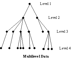
How does aML number data levels?
Does aML support the Cox proportional hazard model?
Does aML support multinomial logit/probit models?
How do I compute predicted multinomial probit probabilities?
What exactly is an observation?
What exactly is a regressor set?
What exactly is a residual draw?
Exactly how are multivariate distributions integrated-out?
ERROR: the maximum dimension of scratch arrays is exceeded -- What to do?
| Q: | What does "aML" stand for? | ||
| A: | Initially, aML was an abbreviation of "applied Maximum Likelihood,"
because we were developing a general-purpose maximum likelihood
optimization package. (All optimization in aML uses Full Information
Maximum Likelihood, or FIML.) We subsequently realized that many users
saw aML primarily as a powerful package for estimating multilevel
models, and only secondarily as a tool for addressing endogeneity and
other problems that require multiprocess modeling. As aML evolved, we
therefore started thinking of aML more and more as "applied MultiLevel."
Back to top. | ||
| Q: | How does aML number data levels? | ||
| A: |
| ||
| Q: | Does aML support the Cox proportional hazard model? | ||
| A: | No, it does not. In practice, however, this is not a limitation. The Cox model
differs from other hazard models in that it does not require you to specify the
functional form of the duration dependency (Weibull, Gompertz, etc.)
This is great, because there is no risk of picking an incorrect functional form.
There are also downsides: Cox's estimation algorithm (partial maximum likelihood)
is less efficient that full maximum likelihood, so that you get standard errors
that are larger than you would get with a parameterized duration dependency. In addition,
the Cox model allows no insight into the duration pattern, i.e., how the hazard varies over time.
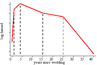
aML requires a piecewise-linear duration dependency (baseline hazard). In other words, the user specifies as many nodes (bend points) as desired, and aML estimates the slopes that best fit the data. Unlike Weibull, Gompertz, etc, this barely restricts the functional form of the duration dependency; it is semi-parametric and will adjust to any pattern in the data. Consider the figure below which shows the baseline log-hazard of divorce as a function of marriage duration, i.e., the marriage duration dependency.
A neat extension, unique to aML, is that it allows for multiple duration dependencies.
For example, the hazard of divorce may depend not only on the marriage duration, but also
on husband's age, wife's age, calendar time, and possibly more concepts of time. Each may be specified
as a piecewise-linear (spline) pattern with its own nodes and slopes. Since all duration dependencies
are piecewise-linear, their sum is again piecewise-linear.
|
||
| Q: | Does aML support multinomial logit/probit models? | ||
| A: | Yes, it does. Version 2 supports both multinomial logit and multinomial
probit models. (Version 1 could estimate multinomial probit models, but
in a very cumbersome manner.) There is no limitation on the number of categories
the multinomial logit can distinguish. The multinomial probit supports up to
four categories (three plus one omitted category).
Back to top. |
||
| Q: | How do I compute predicted multinomial probit probabilities? | ||
| A: |
aML is primarily a package for estimating models, not (yet) for simulating.
It currently does not feature a capability for writing out predicted outcomes,
probabilities, etc. However, you could compute predicted multinomial probit
(and other) probabilities in another software package.
Click here for a discussion.
Back to top. |
||
| Q: | What exactly is a spline? | ||
| A: | A spline is a piecewise-linear transformation of some variable.
Splines play two important roles in aML. First, all duration dependencies
of hazard models must be specified as splines. The
log-hazard is then piecewise-linear or piecewise-Gompertz. The hazard
thus increases and decreases as time ticks on, depending on the signs of
the slope coefficients, as illustrated in the figure above.
Duration splines start life with a "define spline" statement.
Second, you may split up the range of any variable
into segments, and estimate piecewise-linear effects. This is typically
done by transforming the variable using the spline-transformation as
part of a "define regressor set" statement. A spline with n nodes (bend
points) generates n+1 segments and thus n+1 slopes.
Mathematically, there are several equivalent ways to spline a variable.
In aML, the definition is such that the coefficients may be directly
interpreted as slopes on particular segments of the variable (as
opposed to the difference between the current segment's slope and the
preceding one, which would result from a "marginal" spline transformation.)
| ||
| Q: | What exactly is an observation? | ||
| A: | An observation is a set of observed outcomes and explanatory
variables that is statistically independent from other sets. Two annual
wage records of the same person are statistically dependent, need to be
modeled jointly, and are thus part of the same observation. Wage
records of another person (who is not related to the first person) are
independent from those of the first person, and thus part of another
observation. An observation in aML always corresponds to the highest
level, the most aggregated level, level 1. There may be multiple ASCII
records, possibly in multiple ASCII files, pertaining to one
observation. Raw2aml and aML will know that they are part of the same
observation because they all have the same ID.
Back to top. | ||
| Q: | What exactly is a regressor set? | ||
| A: | A regressor set is a vector of variables, say X, which form a
regression equation,  . The
coefficient vector . The
coefficient vector  may be
estimated (or assigned a fixed value). The variables are typically just
variables in the data set, but may be formed as transformations or
interactions of variables. The resulting regression equation may be
used in any model. Think of a regressor set as a may be
estimated (or assigned a fixed value). The variables are typically just
variables in the data set, but may be formed as transformations or
interactions of variables. The resulting regression equation may be
used in any model. Think of a regressor set as a
 , but realize that the
elements of X may be expressions involving zero or more variables.
The variables may be at any level. , but realize that the
elements of X may be expressions involving zero or more variables.
The variables may be at any level.
Back to top. | ||
| Q: | What exactly is a residual draw? | ||
| A: |
Residuals are unobserved and their values for specific outcomes
almost always unknown. While we do not know their values, we do know
which residuals are correlated with each other (multiprocess settings)
and which are equal to each other, i.e., shared by multiple outcomes
(multilevel settings). Correlated or shared residuals are realizations
of the same draw from a distribution. It is essential to
correctly specify which residuals result from the same draw. This is
done with the "draw" feature in residual specifications. Draw
specifications are a nifty way of telling the program which residuals
are correlated and which are independent. See page 333-340 of the
Reference Manual for a detailed discussion.
Back to top. | ||
| Q: | Exactly how are multivariate distributions integrated-out? | ||
| A: |
Where no closed form solution exists, aML allows numerical integration
of normally distributed residuals. As explained in the User's Guide
(pages 103-5 and 274-5 in Version 1, pages 130-2 and 305-7 in Version 2), the numerical
approximation is based on Gauss-Hermite quadrature. The user may choose
the number of integration points; the higher the number, the more
accurate the approximation. The manual illustrates points of support
and their weights for a univariate example and only briefly describes
the algorithm for multivariate distributions:
The points are chosen using Gauss-Hermite Quadrature. Suppose you specify a normal distribution with k dimensions and n integration points in each dimension. aML first computes n standardized points which approximate a univariate standard normal distribution. [...] This method is extended to handle k-variate integration by selecting all nk possibilities of k draws out of n points (with replacement). The appropriate weight for each set is the product of k individual (univariate) weights. These nk sets of points and weights approximate a k-variate standard normal. In order to approximate other k-variate normals (with zero means), aML premultiplies each set of k draws by the Cholesky decomposition of the covariance matrix of the distribution. The marginal likelihood is computed as the properly weighted accumulation of nk conditional likelihoods.The following figures illustrate this approach. Consider numerical integration of a bivariate distribution with six points in each dimension (k=2, n=6). Auxiliary program points, which comes with aML, tells us that the Gauss-Hermite Quadrature support points and weights that approximate a univariate N(0,1) distribution are:
             points       weights
     1   -3.324257E+00  2.555784E-03
     2   -1.889176E+00  8.861575E-02
     3   -6.167066E-01  4.088285E-01
     4    6.167066E-01  4.088285E-01
     5    1.889176E+00  8.861575E-02
     6    3.324257E+00  2.555784E-03
The first figure below shows the support points of two univariate normal distributions, approximated by six points each. The size of the circles is indicative of the weights. 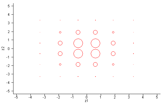 Now let's consider a bivariate distribution with covariance matrix
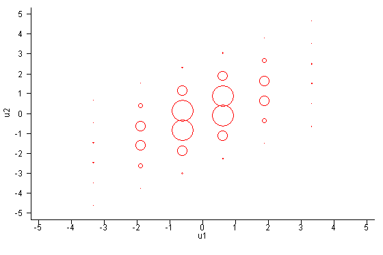 One perhaps undesirable implication now becomes clear. Even though
the bivariate distribution is symmetric in the sense that residuals may
be reversed without consequence, the support points are not symmetric.
Residual u1 is sampled with six unique values;
residual u2 with 36 unique values. This implies that
reversal of residuals in model statements will slightly affect the
results of estimation. Both are approximations and neither is better
than the other. The differences will become smaller as the
approximation improves, that is, as the number of support points
increases.
| ||
| Q: | ERROR: the maximum dimension of scratch arrays is exceeded -- What to do? | ||
| A: |
aML keeps lots of scratch arrays in memory. Some of these, especially
covariance matrices of residuals and their derivatives, can get quite
large when there are very many outcomes per observation. By
default, aML allocates 16MB for such scratch arrays, which is typically
sufficient for up to approximately 600 outcomes per observation. In
rare cases, this is exceeded.
If you receive this error message, you should first make sure that the unit of observation is correct. Do you really have huge numbers of outcomes per observation, or is there perhaps something wrong with the IDs that tie outcomes torgether into observations? Check the data summary information (.sum) file, produced by raw2aml, for number of observations and number of branches within observations. Also check the aML output (.out) file for number of observations and outcomes in your model. Is there really something unobserved that is common to all those outcomes in an observation? If not, re-define your ID variable to refer to a smaller unit. If the data are correctly structured, try running a version of aML that allocates more memory to scratch arrays: bigaml (64MB) or hugeaml (256MB). Run "bigaml" or "hugeaml" in the same way as you would run "aml". These versions support roughly 1,200 to 2,400 outcomes per observation. These larger versions are located in the same directory as your current aml (or aml.exe) executable file. Please be aware that computations involving very large covariance matrices can be very slow. If nothing appears to happen for a while, try a smaller sample (option obs=...;) just to make sure that the bottleneck is CPU resources. If even hugeaml results in the above error message, consider ways to reduce the size of your observations. Can you perhaps ignore unobserved heterogeneity at the top level, or can it be replaced by something observed and captured through (dummy) variables? ("Option huber" generates Huber-corrected standard errors, also known as robust standard errors, which offer some protection against clustering of observations.) Or consider keeping a random subset of outcomes; if you cannot identify heterogeneity with, say, 1,000 outcomes per observation, it is probably not there, and you may re-define observations into smaller units. Finally, beware of aML's default estimates of standard errors. With
very many outcomes per observation, your data may end up having very few
observations. Standard errors are the square roots of diagonal elements
of the parameter estimates' covariance matrix, computed as the inverse of the matrix of
second derivatives (Hessian matrix). By default, that Hessian matrix is
approximated as minus the sum over observations of the outerproduct of
first derivatives (BHHH method). The BHHH approximation is asymptotically
correct, but may be poor in finite samples.
"Option numerical standard errors"
circumvents the BHHH approximation by computing the Hessian as
numerical derivatives of (analytical) first derivatives. Use that
option to obtain more precise estimates of standard errors.
(Perhaps use it for final production runs only; it can be quite CPU-intensive.)
Related, "option numerical search" always computes the Hessian
numerically, not just to get accurate standard errors upon convergence.
| ||
| Q: | I have estimated the effect of a covariate in the form of a piecewise-linear duration spline. How do I test whether it is significantly different from zero at some point other than the origin? | ||
| A: |
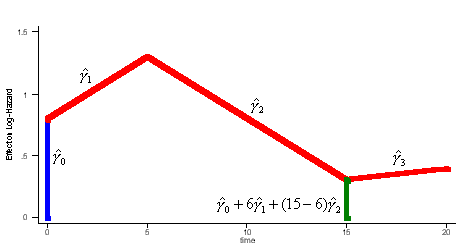 Illustrative Effect on Log-Hazard define spline Effect; nodes = 6 15; intercept;The estimated spline coefficient include an intercept,  , shown in blue, and three slopes , shown in blue, and three slopes
 , ,  , and , and  . The significance of the variable's effect at
the origin is easily determined from the significance of . The significance of the variable's effect at
the origin is easily determined from the significance of  .
But what about at other
points in time? Is the effect significant at, say, time=15? We thus
want to test whether the distance indicated in green, .
But what about at other
points in time? Is the effect significant at, say, time=15? We thus
want to test whether the distance indicated in green,  , is
significantly different from zero. , is
significantly different from zero.
One approach is to derive the distribution of the test statistic:
define spline NewEffect; nodes = -9 0; intercept;Note that we relocated the nodes to be the same as before, but now measured relative to time=15. In the model specification, origin=-15, i.e., 15 years after the beginning of the hazard spell. The two models are equivalent. The estimated slopes will be identical to the original slopes  , ,  , and , and  . The intercept will be equal to . The intercept will be equal to  , and the problem
reduces to a simple t-test. , and the problem
reduces to a simple t-test.
This procedure does not generalize to "kick-in" splines (with "effect=right"), but it does readily generalize to splines that have non- zero origins and to tests at points that do not correspond to nodes. For example, to test whether the effect is significant at time=20: define spline NewEffect; nodes = -14 -5; intercept;Back to top. | ||
Back to technical support
Back to home
 . Its Cholesky decomposition is
 . Premultiplying each pair of univariate
support points by this Cholesky matrix yields support points of the
correlated bivariate distribution:
  . The
figure below graphs these support points.


 . This requires that you know the
variances and covariances of